")
")
FFT analysis
The display of the power spectrum in real time is the most widely used feature of an audio analyzer. The display contains the spectral density over the frequency. The estimation of the spectral density is based on the fast Fourier transform (FFT). The power spectrum display is a very versatile tool.
Typical applications are
- distortion analysis
- frequency measurements
- noise analysis
- measurement of the frequency response
If the input is white noise, you will get a flat display. A widely method to measure a frequency response is using white noise as input signal to the test device. The power spectrum of the output is directly the frequency response.
The power spectrum can be displayed in a line style or as a bar graph display. A more advanced method is the spectrogram to monitor the spectrum over time. You can average several measurements before they are displayed to get a smoother curve. Typical audio analyzers can also display a minimum, maximum or total average simultaneously. You can precisely read measurements from the display with a measurement cursor. The bar graph display is similar to analog spectrum analyzers. It has peak hold and an adjustable dynamic behavior to simulate a fast or slow display. All FFT analyzers have windowing functions to reduce the side lobes. Weighting functions are used to attenuate high and low frequencies to match the measurement with the human ear.
Sample rate vs. block size
The frequency resolution is given by the sample rate divided by the block size of the FFT. For example 44.1kHz and a block size of 1024 the frequency resolution is 43.0664Hz. You can increase the resolution by using larger blocks. But this increases the measurement time. It is impossible to measure with a high frequency and high time resolution at the same time. This is one basic theorem of signal analysis. It can be explained by analog filters. If you implement a narrow filter with high frequency resolution, it's settling time is large. On the other hand, if you implement a fast filter it has a low frequency resolution.
Frequency resolution and FFT size
The frequency resolution is determined by two parameters: the sample rate and the FFT size. Both are linked by a simple equation:
Frequency resolution= sample rate / FFT size
You can easily increase the frequency resolution by using a larger FFT. Typical audio analyzers support up to 16 million points. On the other hand, a larger FFT reduces the time resolution. This is no limitation of the FFT analyzer, instead it is one of the basic signal processing theorems.
We will illustrate this by one example. By default, we use a sample rate of 44100Hz and a FFT size of 1024 points. The frequency resolution is 43Hz and the duration of one block is 20ms. For analysis in the range of 20- 200Hz this resolution is too low. The most effective solution would be to reduce the sample rate, but most AD-interfaces are limited to 32kHz. Therefore, we increase the FFT size to e.g. 16384. This leads to a frequency resolution of 2.7Hz but at the same time the duration of one block increases to 372ms. If you use averaging to reduce noise, you can easily reach a measurement duration of several seconds.
Low frequency measurements are slow.
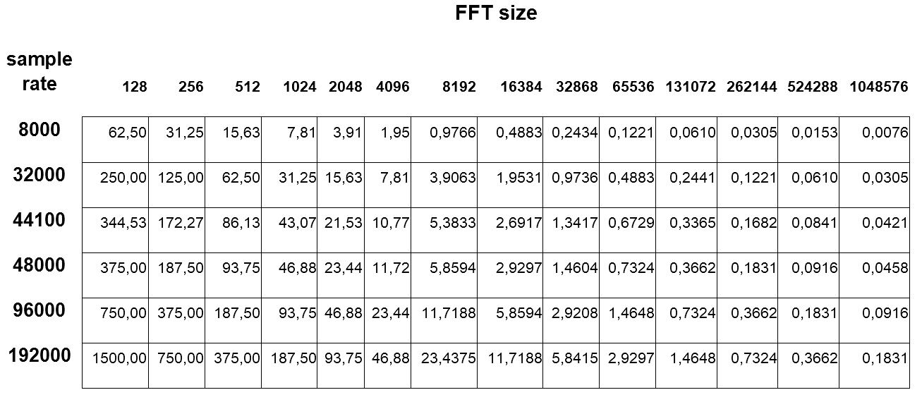
The following table summarizes FFT size, frequency resolution and time resolution for typical sample rates.
Frequency resolution in Hz
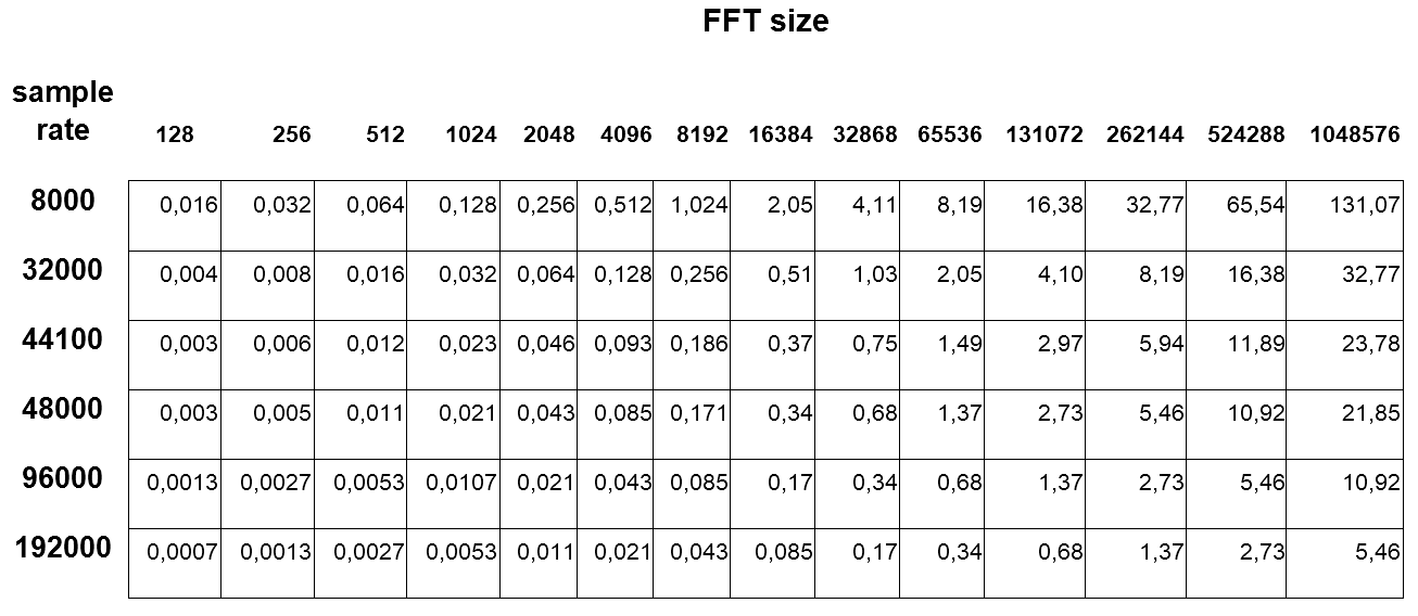
Time resolution in seconds
Windowing
The transformation from the time to frequency domain with the FFT assumes that the input signal is periodic for the block size. Usually, this is only true for sine waves with certain frequencies. At 44100Hz sample rate and a block size of 1024 samples a sine wave with a frequency of e.g. 1378.125 Hz fits exactly into one FFT block. For this case, the discrete Fourier-transform gives the exact spectral representation (one peak at the frequency).
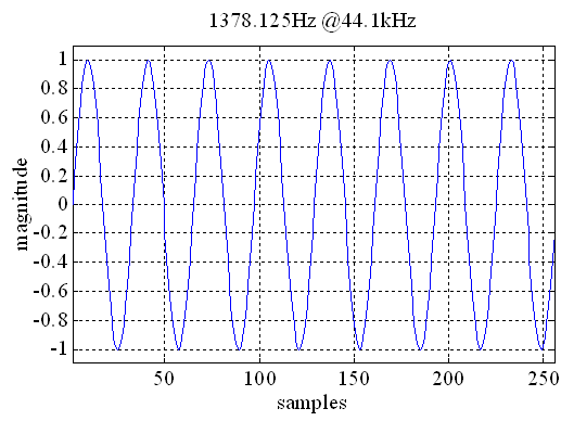
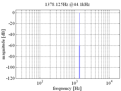
These special frequencies can be calculated easily. F is the sampling frequency e.g. 44100 N is the block length e.g. 1024 n is an arbitrary integer factor f is the cyclic frequency
f=n*F/N n=1;2;3;4 ...
For other frequencies or signals, which do not have this property, there are discontinuities at the transition from one block to another. Although the input signal is a sine wave at a single frequency, the FFT contains level at different frequencies. This effect is known as leakage.
To reduce this effect the input is attenuated at the boundaries of the blocks. This smoothes the differences between periodic and non-periodic continuation. This technique is called windowing. Typical windows are the rectangular window, which does no windowing at all, the Hamming and the Blackman.
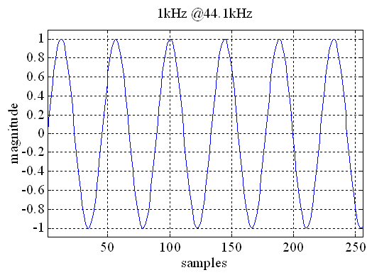
Sine tone at 1kHz. It is not periodic at a sample rate of 44100Hz.
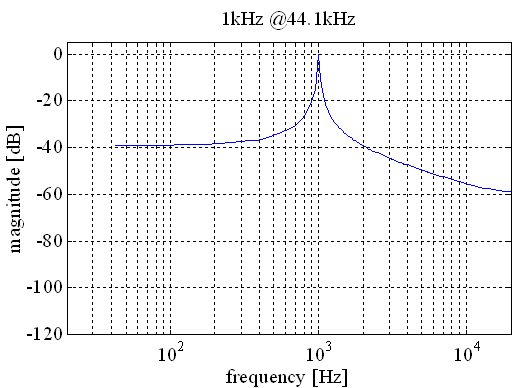
Without a windowing function (rectangular window) we get strong sidelobes. However, we get high frequency resolution.
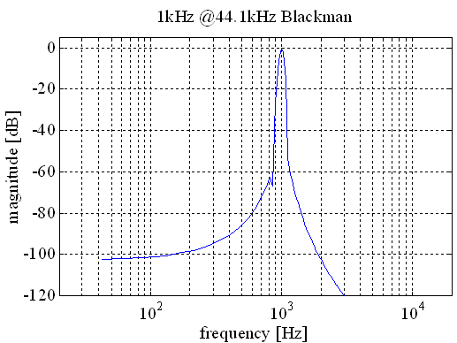
If we use a blackman window, this effect reduces significantly.
Typical audio analyzers support the following window functions:
- Rectangle
- Hamming
- Hanning
- Blackman
- Blackman-Harris
- Gauss
- Flat-Top
- Kaiser-Bessel
- Bartlett
- Rife-Vincent 3-11
The higher the attenuation from the sidelobes caused by the leakage effect, the lower the frequency resolution. The main peak widens. If THD measurements are performed and you cannot use the certain frequencies mentioned above, the best results are achieved with the Rife-Vincent or Blackman windows. However, you get better results if block periodic frequencies are used.
The effect can be demonstrated easily. Set the generator to sine at 1kHz and the analyzer to FFT mode and block size of 1024. The sample rate should be set to 44.1kHz. With the rectangular window set to on, you will monitor sidelobes. If you vary the frequency, you will notice, that at certain frequencies no sidelobes occur. If you use a different window function, the sidelobes are attenuated independently from the input frequency.
Recommendation for window functions
The correct usage of windows requires deep understanding of the theory behind it. If you use a not suitable window, this can have strong impact of the measurement results. For typical scenarios, we recommend the following windowing functions:
- General purpose: Blackman window
- Maximum frequency resolution to measure frequencies: Rectangle window
- Level measurements: Flat-top window
- High side-lobe suppression: Rife-Vincent-5
Typical errors
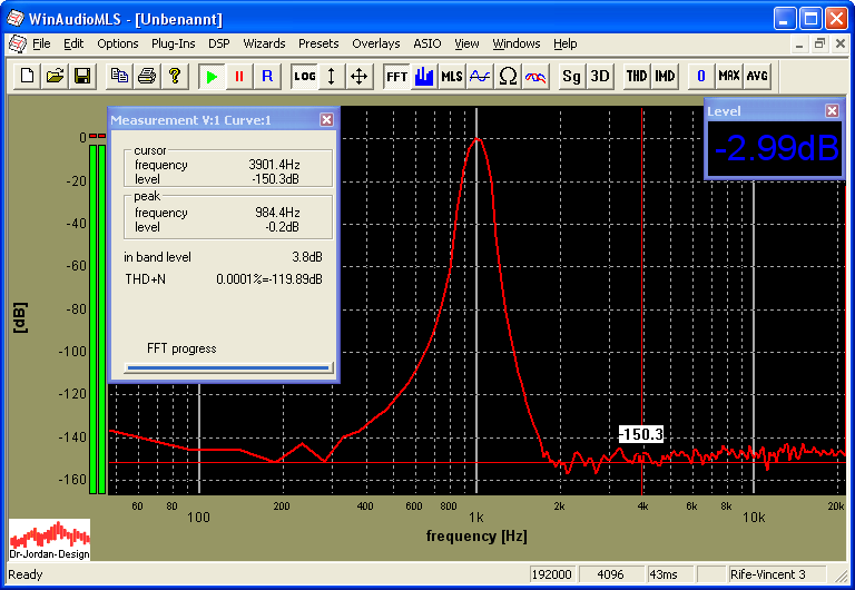
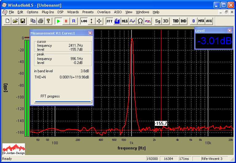
Many people calculate a noise level of –150dB from the following picture, which is resulting to a THD+N of –150dB.
However, this noise level of –150dB is a spectral density, which must be integrated over the frequency range. The audio analyzer WinAudioMLS does this automatically and calculates a correct THD+N of –120dB. This error is clearly visible if we increase the FFT size to 16384. The noise floor reduces to –156dB. We can reduce the noise floor by 3dB if we double the FFT size. However, our noise level is completely independent from any FFT size, therefore it can’t be the noise floor! WinAudioMLS calculates the THD+N correctly to –120dB independently of the FFT size.
Lets’ do the correct calculation:
We assume, that we have a constant spectral density of -150dB at an FFT size of 4096.
The energy for each FFT bin is pow(10,-150/10).
In the frequency range up to 24khz, we have 4096/8 FFT bins. We ignore the few FFT bins for the single tone at 1kHz.
In total we have an energy of 10log10(10^(-150/10)(4096/8))=-123dB.
With a signal level of -3dB, this results to the correct THD+N of -120dB.
